From Making Maps to General Relativity

While I encourage anyone to read this article, some sections assume some familiarity with certain mathematical concepts to keep the article shorter.

There is some familiarity with calculus assumed especially in the section on tangent vectors, and having seen partial differentiation will help there. In addition, some familiarity with vectors and the dot product will help in the section on metrics.

If you aren’t familiar with these concepts, don’t worry! You can skip and reread sections as you like. This article is really about the unexpected power of abstract mathematics.

I hope you enjoy!

“What am I going to use this for?”

It’s a common question in mathematics classrooms and tutorials, and a fair question too. Mathematics is abstract by design, meaning that it does not study any particular concrete real-world thing. Whilst it can make engaging with maths difficult, this abstractness is exactly why mathematics is so powerful, important and interesting.

As an example, I thought I’d try introducing a sub-discipline of maths I find myself studying at the moment.

I just graduated from my undergraduate degree in mathematical physics from the University of Melbourne. This year, I’m taking my first step into the world of research, commencing my master’s research in magnetic confinement nuclear fusion. As I am entering a field of research previously unfamiliar to me, I have been learning about lots of new and interesting mathematics which I will need along the way.

So, without further ado, I’d like to introduce you to…

Differential Geometry

First off, let’s make sense of the name of this sub-discipline: “Differential Geometry”.

You probably have a reasonable idea of what the second word means: shapes and space and stuff.

The first word, differential, is probably only something you’ve heard if you’ve done some calculus before. All you need to know for now is that calculus is the mathematics of change. We use calculus to measure rates of change and how something accumulates if we measure its change over time.

Differential calculus is specifically the branch of calculus concerned with rates of change. So, given some function (a relationship between two quantities - an input and an output), differential calculus arms us with tools to measure how quickly the output changes as the input changes.

So, “Differential Geometry” seems to be the study of shapes and space and stuff using the tools of calculus that let us measure how quickly or slowly things change.

More concretely, we use the tools of calculus to make sense of ideas like lengths, curves and angles on curved surfaces as well as measuring how curved a surface is at any point.

For now, this will do.

Now, I’d like to give you a brief contrast between what differential geometry was originally used for and where it is seen nowadays. Differential geometry is a powerful example of the unexpected usefulness of abstract mathematics.

Early history

The geometry part of differential geometry has been around since ancient Greece. A brief Wikipedia search will reveal that, despite predating calculus by several centuries, the Greeks were clever enough to figure out a few key differential geometry ideas. For example, the ancient Greeks realised that on a flat plane the shortest distance between two points is a straight line, but if you lie on a sphere (such as the Earth), the shortest distance between two points is actually the arc of a “great circle” (a circle whose diameter passes through the centre of the sphere). Already we see that the idea of “distance between two points” works in different ways if you are on a flat vs a curved surface.

Apparently, in 150AD (quite a while ago) Ptolemy (one of the clever ancient Greeks) even came up with what is called a “stereographic projection”, which is also relevant to differential geometry. The “stereographic projection” is a way of associating points on a sphere to points on a flat plane in a smooth way - i.e. to make a map of the sphere.

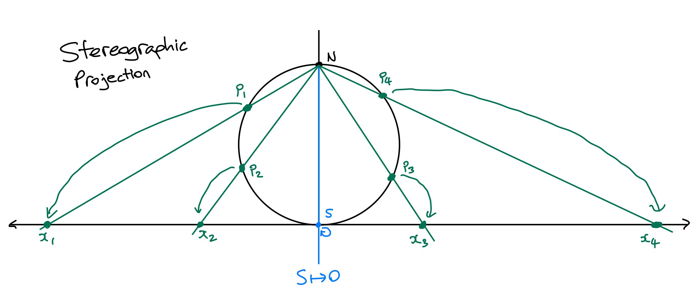
Keeping your eyes on the sketch above I’ll describe how a stereographic projection works. In the sketch we are mapping a circle to a line, but if you want to map a sphere to a plane, you simply map the circle to the line in two directions. First, you pick a point on the circle, let’s say the north-most point (N), and draw the line so that it is tangent to the circle at the diametrically opposing point (S). Now, to map points on the circle to points on the line, you draw a line through your chosen point (N) and the point you want to map. Where this line you draw ends up on the line tangent to the circle is where your point on the circle gets mapped to.

In the sketch above, you see points p1, p2, p3 and p4 get mapped to points x1, x2, x3 and x4. What you may notice is that the point S is mapped to zero on the number line and points close to S are close to zero. Then, as you choose points on the circle closer to N, they get mapped to larger and larger numbers on the number line (compare x3 and x4, for example).

However, the stereographic projection only really works well “locally”, that is, it isn’t a very good map for the entire sphere. If you look carefully at the sketch, you may notice that while S ends up in the centre of our line, the chosen point N…doesn’t land anywhere on our map! The chosen point N is, in a sense, “at infinity” (since numbers which draw close to N become arbitrarily large). This isn’t very good if we want our complete map of the circle or sphere to fit on an A3 page.

So, one of the first ever uses of considering the geometry of a curved surface (in this case the sphere), was to try and make an accurate map of it. Making accurate maps of the surface of the Earth was clearly an important task for navigation in ancient times.

Whilst the stereographic projection is a great starting point, the map couldn’t quite capture every point…especially in a finite piece of paper. This quest of making maps of the spherical Earth continued when differential geometry became a subject of its own in the 1800s, now with calculus firmly in the mathematical toolkit.

Gauss and the Remarkable Theorem

A portrait of Carl Friedrich Gauss by Christian Albrecht Jensen (1840)

I’m skipping over the important historical development of calculus (again, so I can keep it short and get to the really good bit), because I want us to find out why that stereographic projection map was, unfortunately, doomed to fail in the way it did.

In 1827, in a paper called “Disquisitiones generales circa superficies curvas” (which means “General discussions about curved surfaces”) Gauss proved a mathematical result which he called “Theorema Egregium” (which means “remarkable theorem”).

This is what Gauss wrote:

“Thus the formula of the preceding article leads itself to the remarkable Theorem. If a curved surface is developed upon any other surface whatever, the measure of curvature in each point remains unchanged.”

— Carl Friedrich Gauss (translated from Latin)

What does this mean?

When Gauss says “develop a curved surface upon another surface” he means making a map of a surface. So, the particular example of historical interest is making a flat map of the sphere. What Gauss proved is that if you do this, the way your grid lines curve won’t change, no matter how you make your map.

This is why the stereographic projection (and any similar attempt) will never be a completely full and accurate map - the sphere is curved in the same way everywhere…but the flat plane is not curved anywhere! If you try to make a map, the curvature of your sphere can never be fully captured by your flat map.

What is remarkable about this theorem is that it applies to any surface. Even more remarkable is that this property applies to surfaces that don’t even have to exist in real space!

Ok, hang on Nate, what do you mean surfaces that don’t even have to exist in real space?

That’s a great question, dear reader, but let’s park it for the moment so that we can see what crazy stuff differential geometry is up to these days.

General Relativity and the Curvature of Spacetime

You know Einstein right?

If you asked a physicist “what was Einstein’s greatest contribution to physics?” you would likely hear ‘Relativity’ (even though Einstein got the Nobel prize for work on the photoelectric effect).

Relativity is a theory in physics that unites space and time as a single entity: spacetime. Like quantum mechanics, it is extremely well verified experimentally and full of mind blowingly crazy ideas. Relativity falls into two subcategories: special relativity and general relativity.

You can learn the basics of special relativity in high school, it’s actually disarmingly simple. You just take the idea that light moves at a constant speed VERY VERY seriously and then consider what that says about motion when observed from different intertial (non-accelerating) frames of motion.

General relativity…is much harder. You might encounter a few ideas, maybe an equation or two in high school, but to really get to grips with it, one usually takes postgraduate study in physics or mathematics. To put into perspective how weird general relativity is to wrap your head around, it took Einstein about 10 years to get the maths to work, but he had the intuitive notion of general relativity pretty much straight away.

And that’s Einstein we’re talking about.

Well, what’s so confusing about general relativity?

As well as being conceptually very non-intuitive, you have to be able to describe the motion of objects in a curved four-dimensional geometry called spacetime. Four dimensions being strange already, it also isn’t four dimensions in the sense of taking our three dimensional space and trying really hard to extend that image to four dimensions. It’s a four dimensional geometry with some baked in structure which is fundamentally different to how our regular idea of 3D space would work in 4D.

But we’ll get to that later, under “Pseudo-Riemannian Metrics” - which sound extremely complicated right now (and look, I won’t say they are easy or straightforward, they’re not and they’re still well above my pay grade right now) but hopefully the overall idea will make more sense by the end of this article.

The point of this little historical overview (with lots of skipping) is really to highlight how crazy it is that mathematics conceived for the purpose of map making not only told us why we can’t make a perfect map of the globe, but turns out to provide fundamental insights into the nature of space and time.

For now, let me introduce you to some of the basic concepts of differential geometry so that you can gain an overall sense of what’s going on.

Manifolds

In differential geometry, we want to study ‘smooth surfaces’ and we want to try and make little local maps (remember we probably can’t make one full complete map) of this surface which we can use to do calculus, because we know how to do calculus in flat space, so to do calculus on curved surfaces we’re just going to make maps and then do regular calculus on the map.

First things first, we need to decide what constitutes a ‘smooth surface’ which we can do calculus on. Here, we introduce the concept of a manifold.

A manifold is a space which, at every point, there exists a local area that we can smoothly associate with a local area of flat space. Here’s a sketch:

I have my manifold (which I will almost always draw as a doughnut) and around a point x we have a blue ‘zone’ surrounding x in which I have a way of representing this zone in flat space. This zone in flat space is my local map of the zone on the manifold. To be a manifold, I have to be able to do this at every point on the manifold, so x can represent any point.

I could if I wanted, also emphasise that this map gives me a set of coordinates which correspond to the zone on the manifold, however what these coordinates look like may vary as I move around the manifold. Here’s another sketch where I fill in some green grid-lines.

Now, keep in mind that this is abstract maths so details like the size and shape of the zone around x and the method I have of making a local map are not important, for now we just care about whether it can be done in principle.

There are a few symbols going on in my sketches which I’ll give definitions for below. Mathematicians use lots of symbols because once a definition is established it’s much quicker to draw one symbol than write the whole thing out again.

Note: if I ever use the term “Euclidean space”, what I mean is “normal” space in the way you are used to. That is, whatever you think right now about how “space” works (parallel lines never meet, internal angles of a triangle add to 180° etc.) is how “Euclidean space” works, but there are plenty of spaces which don’t work like this. As a simple example, triangles drawn on a sphere can have interior angles which add up to anywhere between 180° and 540° (non-inclusive).

The next important question to ask is: “How do I navigate between different zones which have different maps?”

Here, we add an additional requirement to the manifold called a smooth structure.

If any two zones overlap (And they will, because every single point on the manifold have these zones), the overlapping region has two different maps of it, given by the two different zones.

A smooth structure is the requirement that, when this happens, I can ‘smoothly’ move between the two different maps.

That is, the two different maps are just two different regions of flat space, and I can move between these regions in a smooth way (so no tearing, crinkling, glueing or ripping space, think just smooth moulding of clay).

Here’s another sketch:

I have two different blue zones which have two different blue maps. The overlapping region is in green, and the green arrow is my way of smoothly moving between the two different maps. There are some more symbols here, so I’ll define them below:

In the above, think about the symbols representing the maps as “actions” I can take. So my map of U is an action where I take the zone U and follow the map to where it ends up in flat space. I can then do this action backwards to trace a map back to a zone on the manifold. The transition map which I define above is a combination of two actions: first trace the map of U back to U then follow the other map to V.

Keep in mind that all this stuff about things being “smooth” is stuff we already understand in flat Euclidean space (thanks to calculus), we just want to extend it to not-so-flat manifolds.

Once we give a manifold a smooth structure, we call it a smooth manifold, which hopefully seems reasonable.

Functions between manifolds

So we know the kind of spaces we want to look at. We want spaces that have these little zones which you can make maps of. Another way to put it is a space that if you zoom in enough, looks pretty much like flat space. Additionally, we want these manifolds to have maps that glue together well (that’s the smooth structure).

That’s just our space though. The next thing we probably want to make sense of is how functions on this space work.

In high-school calculus, we do calculus with functions so that we can find rates of change and maximum and minimum points and all that. So, we have our space but we need to understand how to think about functions on this space.

Further, we want to do calculus with these functions. This probably wasn’t mentioned in high school calculus, but you can only do calculus with some functions, not all of them. You need the function to be “smooth” (notice that term again).

If you don’t believe me, think about taking the derivative of the absolute value of x ( f(x)=|x| ) when x is zero. It won’t work.

The first thing we consider is functions where the inputs are points on a manifold, and the output are points in flat Euclidean space. This is a helpful stepping stone.

Again we already know how smooth functions work in flat space, so the trick will be looking at our function with our local maps which are flat.

A function from a manifold to some flat space is called smooth if, for every local map of the manifold, the composite function which takes points from the map back to the manifold and then to the output flat space is a smooth function. It’s a lot of words (this is why maths uses a lot of shorthand symbols instead), so read it carefully and follow along on the picture below:

That bit about “takes points from the map back to the manifold” is the ‘reverse action’ of making our local map. Remember at every point we have a zone with a map. We can also take points on the map and trace them back to the zone. To make things easier, I’ve written out what some of the symbols mean below:

Now we can extend this definition to smooth functions between two manifolds. Let’s say the function takes points from a manifold M to a manifold N.

It works exactly the same way. The function between manifolds M and N is smooth if for any two chosen zones, the composite function which takes points from a map of M back to M then through to N then through to the map of N is a smooth function. This composite function (which has three steps) is just a function between two flat spaces, so our already understood flat-space notion of smoothness applies!

If things are getting a bit confusing here, don’t worry, that’s fine. Here are some definitions of symbols below which may help clear things up:

Focus again on the pictures and notice the common thread. We have a space that has all these local maps of it that glue together well and use the maps to understand the functions.

To make sense of calculus on manifolds, what we do is look at the maps, rather than the manifold. That way, we can use our already tried and true methods of calculus made for flat space just by adding an extra step of turning local areas on manifolds into maps. If you wanted to differentiate such a function on a manifold, you would essentially just differentiate the coordinate representation of the function using the map of the local area you’re in.

Again, you don’t have to understand every bit of what I’m writing. What I hope is that you are picking up on an overall flavour of differential geometry and how it works, and perhaps getting a picture of why it is so powerful and has such an interesting history.

Tangent vectors

Next up, if we want to talk about calculus, rates of change, motion of particles and all that on these manifolds, we are going to need to have a sense of direction at each of these points. Here we introduce an idea of tangent vectors. It is important that we have a sense of direction at a particular point on the manifold because as we have already seen, the ‘maps’ we use to make sense of manifolds usually change from point to point, so the same will likely be true of our sense of direction.

Here, things can begin to get a bit strange and especially abstract, but let’s have a go anyway.

A reasonable initial attempt at making sense of directions in space at a given point on a manifold is to consider vectors that are ‘tangent’ to the manifold at a certain point. So, for example, my doughnut manifold in 3D space (which I am very fond of) will have, at each point, a flat plane (like an unbendable sheet of paper) which sits on the manifold at precisely that point.

However, mathematicians aren’t particularly fond of this way of defining tangent vectors. This is because it only works for Euclidean manifolds. That is, manifolds which ‘sit inside’ regular Euclidean space (even though they may be however-many-dimensional, they still behave like our 3D space in important and specific ways). Mathematicians want their theories to apply in as many different situations as possible (mathematicians are forever in search of the ‘general case’). So, mathematicians will want this tangent vector notion to work for some other, much stranger spaces than just spaces which behave like our 3D space.

So, how do we define a sense of direction on our manifold without using a plane tangent to the manifold?

There are a few equivalent ways of setting it up and each are fairly abstract and weird at first but have their own list of pros and cons. I will introduce you to one of them, where we utilise a multivariable calculus notion of directional derivatives to create our tangent vectors.

Directional Derivative

In high-school calculus, we learn how to take the derivative of a single-variable function and find that this tells us about the rate at which the function value changes as we change the input value.

In a university calculus course, we learn how to extend this method to functions with multiple variable inputs, and it is not a significant leap in difficulty.

Firstly, a quick note on visualisation. A function of a single variable can be visualised as a graph where the horizontal axis represents possible input values and the vertical axis gives the corresponding output values.

If we wanted to consider a function that takes two inputs and produces a single output, we could imagine a 3D space where the x-y plane represents all possible combinations of our two inputs and the z axis gives the output of the function. Here, we have a visualisation something like the topography of some mountains, where at any location the height of the hills and mountains correspond to the output of this function.

Visualisation gets trickier in higher dimensions, but all the principles remain the same.

When we have these multivariate functions and we want to take a derivative, we have the added complication that we need to specify in which direction we would like to take the derivative. After all, functions of more than one input may change at different rates in different directions.

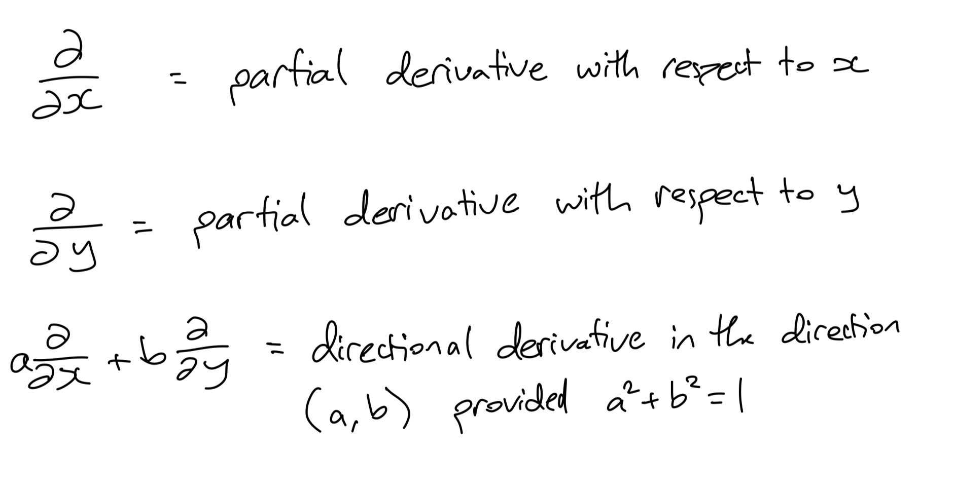
So, we take what we call partial derivatives, where we pick one variable to differentiate and leave all the others as if they are some fixed value. Visually, this corresponds to taking some slice along a particular direction (the dotted lines below), where the slice we pick depends upon the value we fix the other inputs to be.

We can then take sums of partial derivatives as a way of specifying a directional derivative.

In a university calculus course, you may learn to do this by taking an inner product (which we’ll meet again later) between a vector (the direction we want to differentiate in) and a gradient function, which is a new function that stores the rates of change in all directions.

Now, what I want to point out is that these directional derivatives are all different ways of differentiating some multivariate function, and while the result may depend upon the function, the directional derivative is really it’s own entity.

If we omit the specific function f we are differentiating, we can observe the remaining symbols as a representative of this separate entity, which behaves in a consistent way when acting on any particular function

Indeed, this entity is an example of something we might call an operator, a mathematical object which acts on other mathematical objects in some consistent way. For example, high-school calculus differentiation is an operator which acts on single variable functions. Indeed, addition and multiplication can be thought of as operators which act on pairs of real numbers. In both cases, the result changes depending on the object acted on, but the operator has some of its own consistent behaviour which we can separate from the results of it’s actions on objects.

Not only are these directional derivatives independent entities, but they are entities which contain specific directional information. However, these entities don’t require manifolds which look like regular 3D space, because so long as you have a local flat map (which you always do on a manifold, this is after all what makes it a manifold), you can make sense of partial derivatives on a manifold by taking partial derivatives on the flat map!

So, we have a great candidate for tangent vectors which work for any manifold.

Tangent Vector

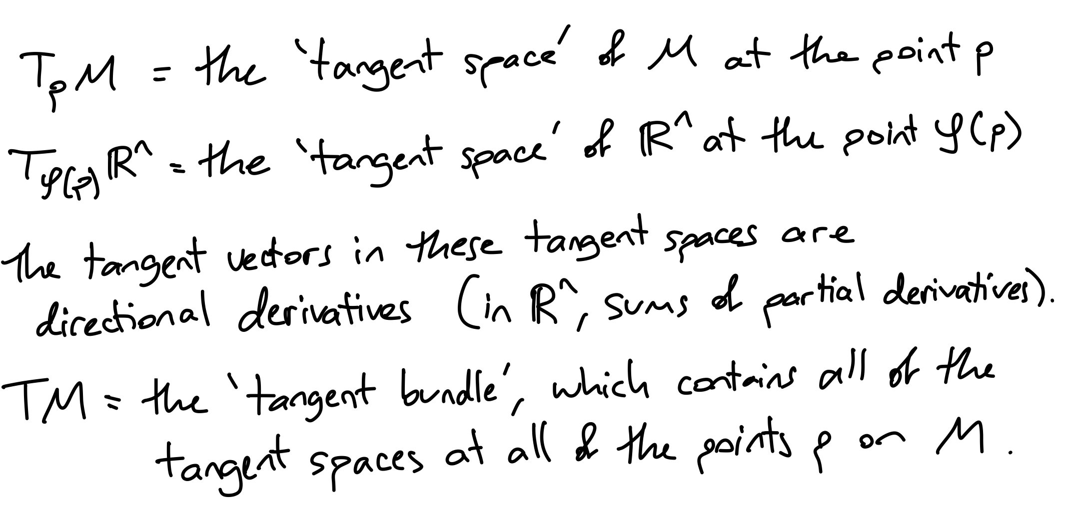
So, one way we can define these tangent vectors (which we would like to use to make sense of directions on our manifold) is as whatever partial derivatives on our maps look like on our manifolds. What do I mean by this? Well, just like how we made sense of functions being smooth by looking at whether they are smooth on all of our maps, we can take partial derivatives on our maps and trace them back to our manifold. By doing this, we can use partial derivatives in flat space (which we already understand) and translate that knowledge onto the manifold (by tracing our map back to the manifold). Here’s a few symbols to condense what I am saying here:

So now we have all the tools to convert regular calculus in flat space to calculus on a manifold.

The common thread to recognise throughout all this is that we have carefully designed tools to do calculus on a manifold primarily by taking what we already know about calculus in flat Euclidean space and translating it onto these manifold objects via our maps (which are one of the defining characteristics of the manifold).

Another way I could describe a manifold is as a ‘space smooth enough to do calculus’. What we really mean by this is that at every point in this space we can translate the local area into flat space, and do calculus there before translating the effect back.

Metrics and Riemannian metrics

Now let’s introduce some geometry into our calculus on manifolds.

In my undergraduate maths degree (and many similar degrees with scientific or engineering components) the first year maths requirements broadly fit into two categories: calculus and linear algebra. Linear algebra is often a student’s first encounter with lots of pure mathematics, abstraction and theorem proving. This kind of maths has a very different feel and skillset to computations and calculations that dominate high school mathematics study. It is in this subject that I first encountered the power of abstraction and how we can use maths to give precise definitions to our intuitions for certain ideas, and from the precise definitions make new discoveries that our intuitions could never have come up with.

One particular abstraction students learn about in linear algebra is that of inner products between vectors.

When we first learn about vectors (arrows in space…at first), we seem to have a built in sense of their geometric properties: how long a vector is and at what angle it is directed relative to other vectors. This is because our first example of vectors is 3D space as we are used to it, which actually happens to have a lot more structure than just the structure required to make precise our notion of vectors.

Students come to learn that you can define and play with vectors without having any sense of their length. For example, functions such as polynomials behave in every way required for us to call them vectors, but if I ask you “what is the angle between x² and x³”, it seems like this question has no meaning! We can however make sense of this question if we introduce an additional set of rules to the rules followed by vectors.

What we do is we introduce a way of taking two vectors and multiplying them to give us a single number. As with all abstract maths, the exact way we do this is not important, so long as it follows a few rules:

multiplying a vector with itself must not give a negative number and can only give zero if the vector is the zero vector
the order you multiply doesn’t matter (we call this symmetry, if we use complex numbers we actually need conjugate symmetry which is slightly different)
the multiplication is linear (for now, all you need to know is that multiplying sums of vectors is just like multiplying sums of numbers in brackets)

If your method of multiplying vectors (however it works) satisfies these rules, we will say it is an inner product.

Here’s a sketch of what information inner products give. In a broad sense, it tells you something about how much two vectors ‘overlap’. If they don’t overlap at all, the inner product will be zero, while if they are completely overlapping, the inner product will be the product of the lengths of the vectors.

Once you have an inner product you can make sense of lengths and angles between vectors using formulas that involve inner products. As an example, when you first learn about vectors in Euclidean space, the inner product of choice is the dot product

So, if you have an inner product between polynomials (the usual choice is an integral of the product if you wanted to know) you actually can, if you really wanted to, say what the angle between x² and x³ is.

This may seem silly right now, but some of the most useful advanced mathematical tools entirely rely on the fact that this works and makes sense. Tools such as Fourier series, which enable us to solve and model complex engineering and physics scenarios, require us to take inner products and define lengths of trigonometric functions!

Ok…but what does that have to do with our map-making?

Well, we have so far this sufficiently smooth space that we can locally make (flat) maps of which we can read well (because we understand lots about flat space). We use these maps a lot to make sense of how things work on the manifold, and we have made sure that if we move around this space, our maps move around in a smooth and understandable way (no sudden teleporting!)

If I want to start defining geometric ideas such as the length of some path or the angle between lines on my manifold, I am going to need the mathematical tools to express length and angle…that is, an inner product. Well, what I am actually going to use is a metric, but for now just think of this as an extra slight abstraction of an inner product. That is, every inner product is a special kind of metric, but metrics don’t need to be inner products. So if you’re confused but understood the inner product idea, just replace metric with inner product and you are still fine, there are just other cases where this isn’t true and everything still works.

A Riemannian manifold is a smooth manifold (it has everything we have built so far) with the additional structure of a Riemannian metric. A Riemannian metric is essentially a choice of metric at every point on the manifold. That is, once you pick a point, at that point it works just like a metric, but since our manifold’s map can change from point to point, the specific choice of metric we use at each point is allowed to change just like our maps.

So, as an example, here is a sketch. On the left I have flat space and I have a metric defined on the whole space. On the right I have a manifold, where two points each have a metric but the metric may or may not be different.

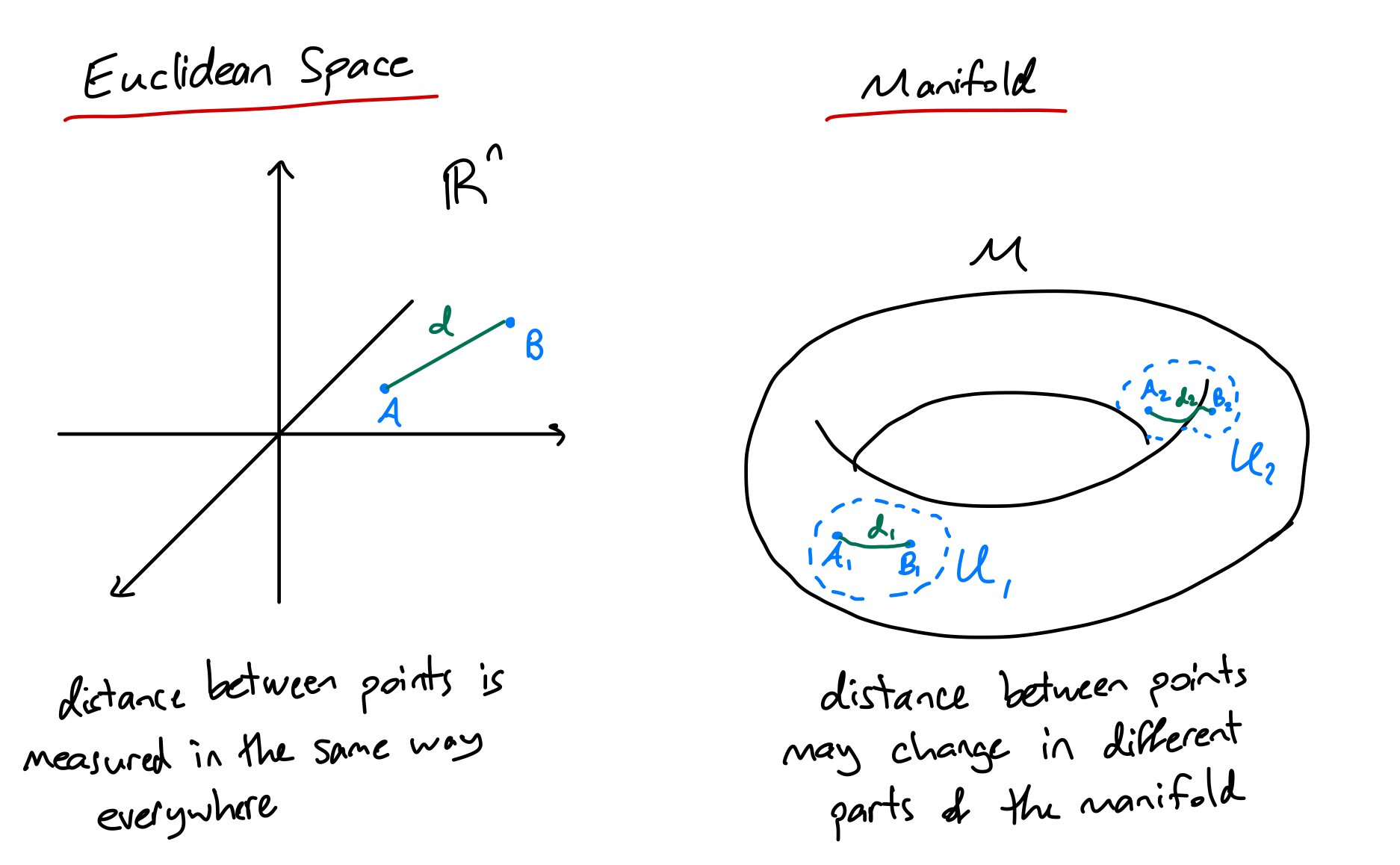
Again, since our manifold’s maps change as we move in a coherent way (the smooth structure), the metric we choose also has to change in a coherent way (some distance can’t be length 1 somewhere and suddenly instantaneously length 1 million right next-door).

If you’re still following, great job! Really, this is weird abstract stuff. Now, I have skipped over a lot of work required to really properly make sense of Riemannian metrics (tensor fields, covariance and contravariance, differentials etc. etc.) but I hope you at least walk away with two things:

an overview of what we are trying to do in differential geometry
an appreciation for the process of pure mathematics and abstraction

Once you have all this structure built up of manifolds, smooth structures, tangent vectors and everything needed to define Riemannian metrics, you can do all sorts of calculations (like calculus) on these Riemannian manifolds. These calculations are what give us things like gravity as the consequence of curved spacetime in general relativity and calculating transport and motion of plasma particles in magnetic confinement fusion devices.

Some General Relativity: Pseudo-Riemannian Metrics

Now after all this discussion, are we ready for general relativity?

Well, as I mentioned earlier there is an additional fundamental difference in the structure of spacetime compared to just adding a fourth dimension to regular space.

In our mathematical structures this means we remove some of our requirements for a more general structure. Instead of requiring a Riemannian metric, we require a slightly more general object called a pseudo-Riemannian metric. The key difference is in how we measure length in a space which includes time rather than just space which includes space. That is, in 4D spacetime, we have three dimensions of space and a dimension of time which behaves a bit differently.

There is a complex discussion to be had here, which is above my pay grade, for now I just want to point out the physical principle which translates into this generalisation of the metric structure. It comes down to the motivation for spacetime.

In special relativity, we see that the time an event takes or the distance between two points can actually change depending on how fast the observer of the event is moving relative to the speed of light - distance contracts and time dilates the faster you move. This is tricky to deal with, so we want a space in which something (not necessarily distance or time) doesn’t change depending on your perspective. This thing which doesn’t change is called the invariant interval or the spacetime interval and ends up as our length measurement in spacetime. However, this interval isn’t quite the same as distances between points in regular space.

In regular Euclidean space, the square of the distance between two points is just the square of the distance between their coordinate components (think about Pythagoras’ theorem and notice the similarity):

When we include time as one of our coordinates (as we must when talking about things in spacetime) the sum of squares of components changes between observers moving at different speeds:

What turns out not to change is instead the following interval:

So this quantity won’t change between observers moving at different speeds. So, it is instead this interval which becomes our measurement of length in spacetime.

The fact that some terms are positive and some are negative is what makes our metric pseudo-Riemannian instead of just Riemannian. If all the terms were positive it would be Riemannian.

Again, there is a lot of important detail I’m brushing over so don’t worry if a lot still doesn’t make sense (you and me both, dear reader). All I hope to point out is the interplay here between physics and mathematical structure: the observation that there is an interval of spacetime that doesn’t change between observers manifests in our mathematical structure as a relaxation of what we consider a reasonable basis for defining lengths and angles.

Conclusion

Ok, I think that’s quite enough skimming over details in complicated maths. I hope you enjoyed the read, and I apologise in advance if some discussions left you more confused than before.

I hope however, that I could communicate the following:

Mathematics, at the tertiary level and beyond, is not just concerned with ever more complicated calculations, but also with how we can make precise our intuitions for how things work.
Abstraction is a very powerful tool that can lead us from our intuitive understanding of the world around us to deep insights about the structure of the universe and the structure of logical reasoning that we could have never imagined before.
If you want to make a map of the Earth, good luck, it will inevitably be a little bit distorted somewhere or other because spheres are curved and flat pieces of paper are not
By studying objects and structures without any particular concrete example in mind, maths is able to contribute valuable insights to radically different fields at the same time!

Finally, if you enjoyed this article or you have any feedback or constructive criticism you would like to give me, feel free to reach out! I hope this was enjoyable and I hope to improve my writing through this practice.

If you’re interested in online tutoring for years 7-12 or undergraduate-level mathematics or physics, you can book here.